

3D Steam Turbine Flutter Test Case
Introduction
The geometry and steady flow conditions of this test case is the same as the Durham University Open 3D steam test case . This geometry was chosen because it is the only open 3D geometry for a steam turbine stage that we are aware of. The scale of the geometry and prescribed flow conditions are similar to a typical working steam turbine. To create a flutter test case we have simply defined the material of the rotor blade to be steel and it is assumed that the rotor blade is fixed rigidly to the hub.
Geometry
The main parameters describing the geometry of the test case are listed in the table below
| Number stator blades | 60 |
| Number rotor blades | 65 |
| Length rotor blade | 920 mm |
| Speed of rotor | 3000 RPM |
| Stagger angle at tip of rotor | 67 degrees |
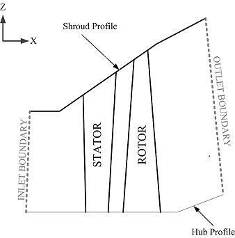
A schematic of the flow domains is shown below.
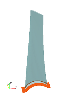
The rotor blade is shown below.
Data Files of Geometry
Zip file of iges files of geometry (zip 92 kB)
Flow Boundary Conditions
The prescribed inlet condition for the stator are listed in the file below. All flow condtion are in SI units (metres, Pascal and Kelvin). The flow angles are in degree. The inletAlpha is the atan (circumfertial velocity component / axial velocity component) and inletBeta is the asin (radial velocity component / magnitude of velocity). The average inlet flow conditions are total pressure 27 kPa and total temperature 340 K, and the average isentropic exit Mach number is 1.12. These conditions are typical for the last stage of steam turbines. The flow is transonic at the rotor tip.
We have decided to set a constant static pressure 8800 Pa at the diffuser exit.
Calculation of Mode Shape and Frequency
The geometry defined for this test case is the hot or the aerodynamic geometry. This is the geometry of the blade when the rotor is spinning at 3000 RPM and with the aerodynamic forces at the prescribe operating point. In order to correctly calculate the mode shape we need to calculate the cold geometry, that is the geometry when the rotor is not spinning and without aerodynamic loads.
The blade is assumed to be a free standing blade made from steel which is rigidly fixed at the root. The properties of the steel are shown in the table below.
| Density (kg/m^3) | 7750 |
|---|---|
| Youngs Modulus (GPa) | 210.0 |
| Poisson's ratio | 0.3 |
The rotor speed is 3000 RPM. The blade geometry in the IGES files above is the hot geometry. In order to properly calculate the mode shape it is necessary to determing the cold geometry. This can be done iteratively. Pre-stress and spin softening are both considered in the modal calculation. The flutter analysis is performed for the first bending mode. The natural frequency of this modal shape calculated by ANSYS is 92.953 Hz, which correspond to a reduced frequency of 0.2.
The data file for the calculated mode shape of the first bending mode is below. This mode shape was used for all unsteady flow simulations. The mode shape has been normalized so that U^T M U = I. The average kinetic energy of the blade in one cycle is 0.25 omega **2, where omega is the circular frequency when the blade is oscillating at the normalized amplitude.
firstBendingModeShape.zip (zip 1,1 MB)
Post-processing
In order to compare solutions from different codes, a consistent method of extracting solutions is required. Solutions are usual compared at a fixed span height. The location of the span surface for a give span percentage is shown in the figure below.
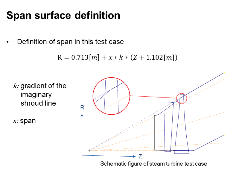
Steady Solutions
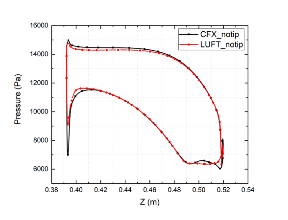
Plots of steady-state pressure on the rotor blade at 50% and 90% span calculated by LUFT and CFX are shown below.
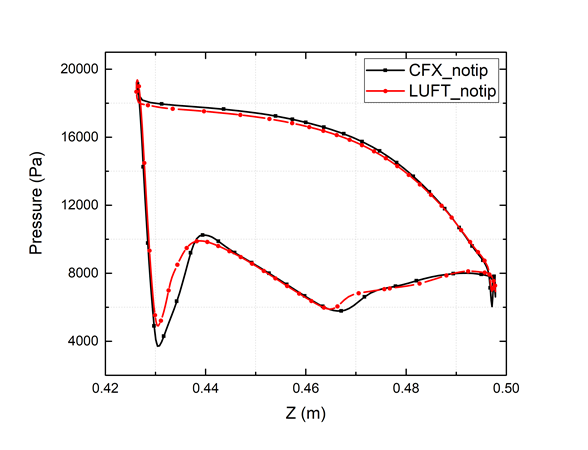
The data files for the LUFT steady-solutions are below
LUFT_SteadyStateSolution.zip (zip 19 kB)
Unsteady Solutions
Unsteady flow simulations were performed using LUFT. The harmonic motion of the blade was prescribed as the first bending mode (data file above) at all possible nodal diameters. The modal frequency was adjusted to 132.08 Hz in order to increase the reduced frequency to 0.3 which is typical for steam turbines in use.
The plot of logarithmic decrement versus nodal diameter calculated by LUFT is shown below.
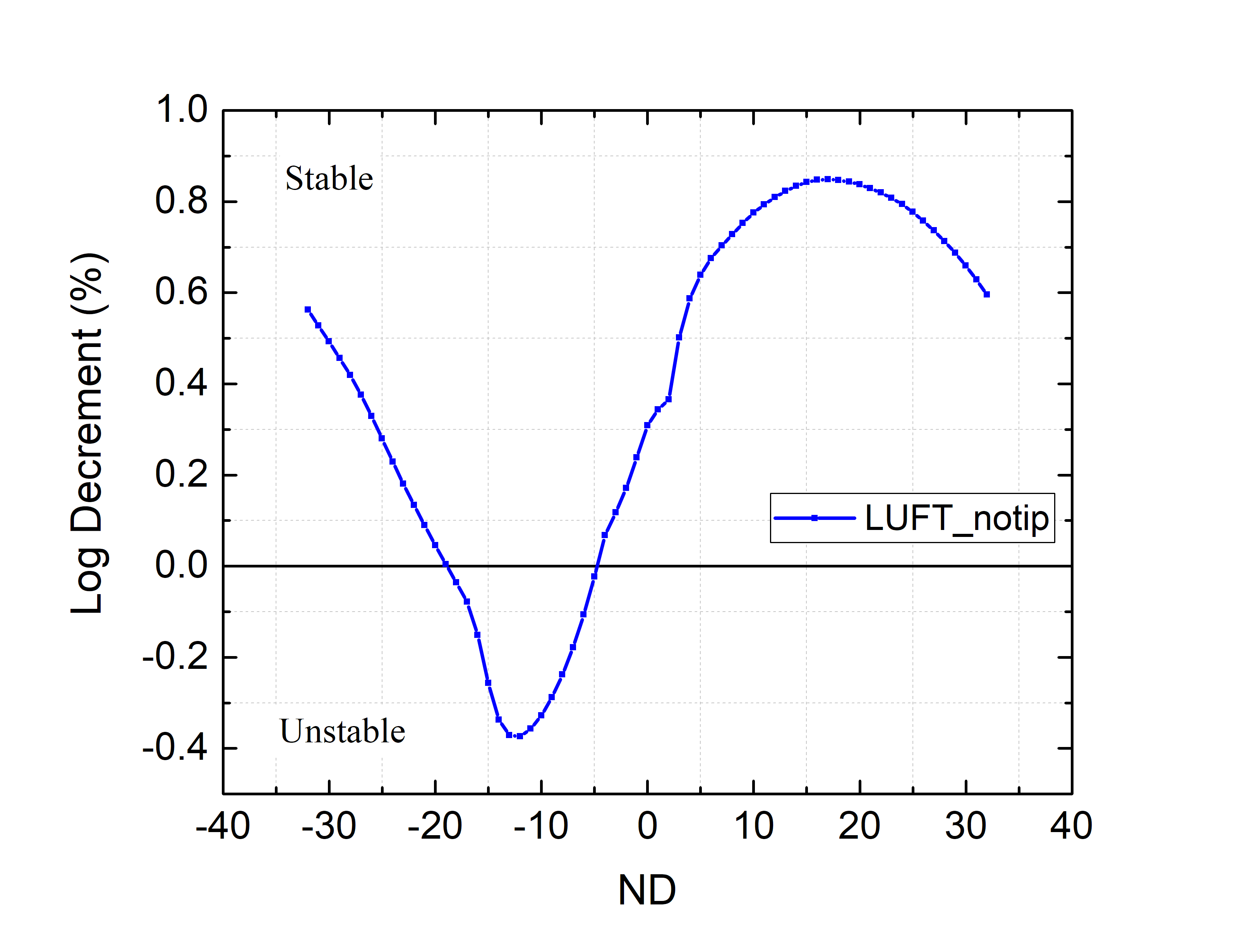
The data file for logarithmic decrement is below.
The plot of the local work coefficient at IBPA = -45 is shown below. Note that IBPA0-45 degrees does not correspond to one of the possible nodal diameters. This IBPA was chosen because it is easier to calculate this solution in the time domain (8 blade passages).
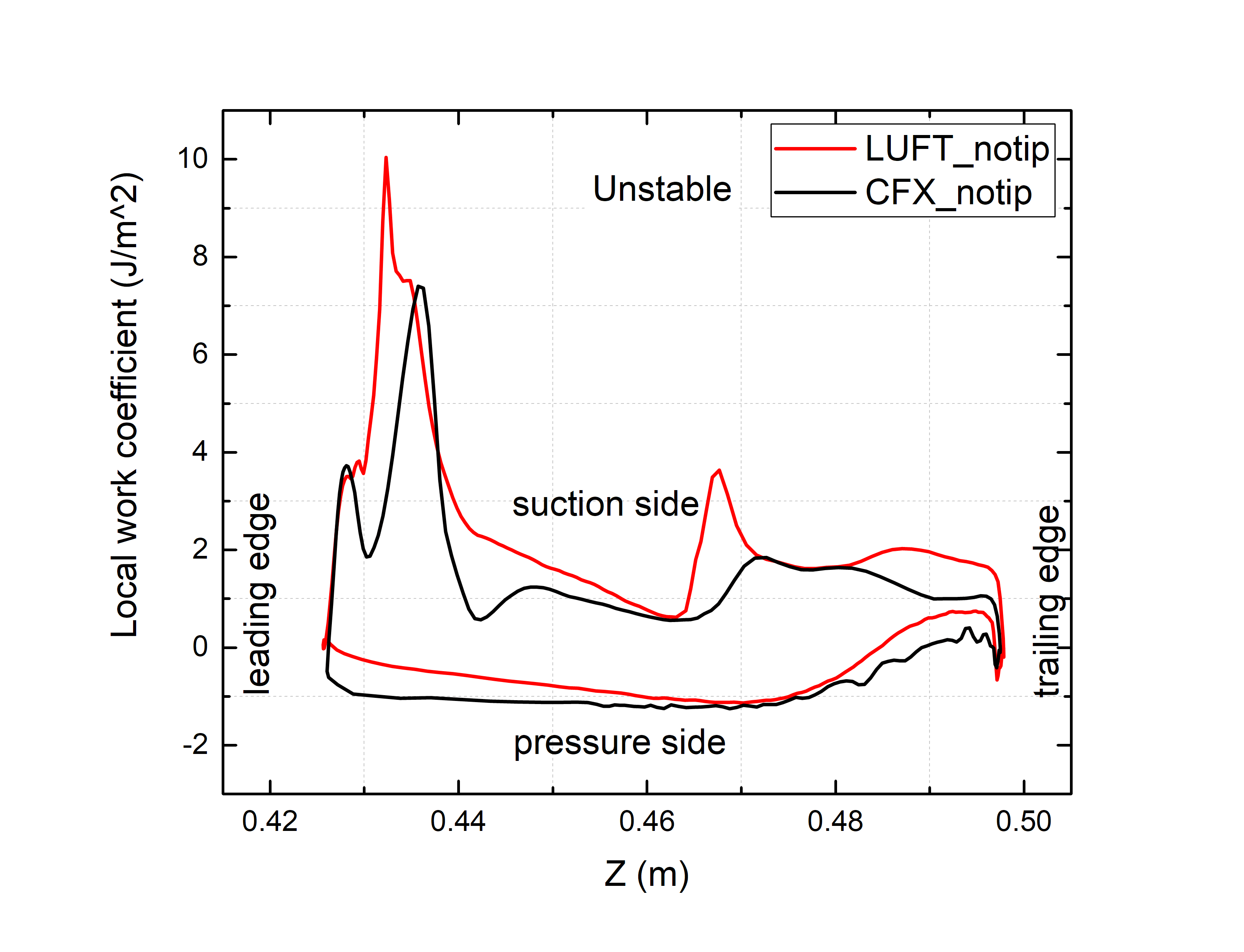
The data file for the local work coefficient is below.
luftSolutionIBPA-45span90 (txt 5 kB)
Publications
Establishment of an Open 3D Steam Turbine Flutter Test Case (pdf 703 kB) by Qi Di, Paul Petrie-Repar, Tobias Gezork, and Sun Tianrui, published in the Proceedings of the 12th European Conference on Turbomachinery Fluid dynamics & Thermodynamics ETC12 April 3-7, 2017: Stockholm, Sweden
Investigation of Tip Clearance Flow Effects on an Open 3D Steam Turbine Flutter Test Case by Sun Tianrui, Paul Petrie-Repar, Tobias Gezork, and Qi Di, to be published in the Proceedings of ASME Turbo Expo 2017: Turbine Technical Conference and Exposition GT2107, June 26-30, 2017, Charlotte, NC, USA